Teledyne Hastings Instruments Blog

Over the next several blogs, we will be discussing various industrial gases. While some of these (carbon dioxide, argon, methane, and hydrogen) may be very familiar to our readers, other gases may not be as well known. In this blog, we will take a look at sulfur hexafluoride (SF₆), a gas that is one of the most important today in the utility industry.

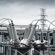
SF₆ is an interesting gas primarily because of its electrical properties. Certain neutral gas molecules can easily capture free electrons and form stable negative ions. The efficiency of negative ion formation in a gas is determined by its electron affinity. SF₆ , it turns out, has a very high electron affinity and therefore has excellent electrical insulating strength. So, in an electrical discharge inside a volume containing SF₆ gas, the free electrons generated by the discharge are captured by neutral SF₆ to form negative ions. These large negative ions are not able to travel quickly and so the discharge is usually quickly extinguished. One other note about SF₆, the insulating property of the gas improves with increasing pressure. SF₆ is colorless, odorless, non-toxic, and non-flammable. As you can see, these properties make it very useful to the generation, transmission, and distribution of electricity. 80% of the world’s SF₆ gas is used by electrical utilities in circuit breakers, transformers, and gas insulted switches.

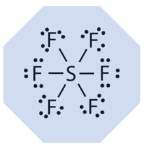
SF₆ is arranged in a hexagonal structure. Each of the six fluorine atoms shares two its electrons with the outer shell of the sulfur atom in the middle. This structure gives SF₆ its stability over a broad range of temperatures; the gas is thermally stable up to 500°C.

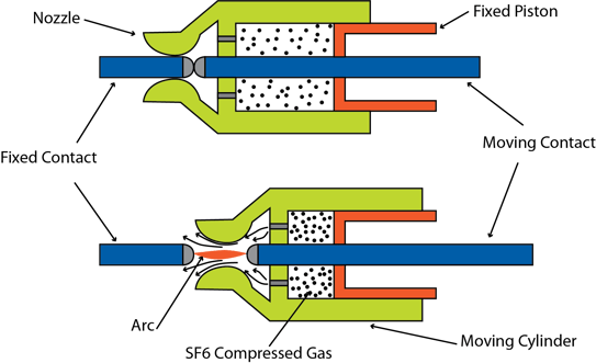
SF₆ is often used in high voltage breakers. One example is the so-called dead tank breaker. In a dead tank breaker, the tank is electrically tied to earth/ground. In the live tank version, the tank is floating at a higher voltage.

The “make/break” mechanism of the breaker is shown in the diagram below. As noted above, the insulating properties of SF₆ are improved with increasing pressure. So one of the jobs of the breaker’s piston actuation is to compress the SF₆ gas and force it to flow into the arc region. As the contacts are moved apart, current will try to continue to flow as an arc. Any resulting arc is quickly extinguished by the pressurized SF₆ flowing into the region. Incidentally, during breaker manufacturing, vacuum gauges from Teledyne Hastings are used to measure vacuum levels inside the vessel during pump down as the air is removed. After evacuation, the region can be filled with SF₆.  

OK, one last note about SF₆ to conclude this blog and this falls under the category of “Don’t Try This at Home.” Just like Helium will make your voice sound higher if inhaled, SF₆ will make your voice sound lower. You can find many demonstrations of this on YouTube. The most famous example is probably the demonstration on “The Big Bang Theory.” However, SF₆ is one of the most powerful greenhouse gases and its release into the atmosphere should be minimized.

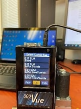
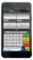
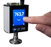
Teledyne Hastings builds both vacuum and flow instrumentation which can easily work with SF₆. Note that SF₆ has a very high thermal conductivity. Conceptually, this makes sense because the gas molecule has many degrees of freedom – translational, rotational, and vibrational.  The GCF (gas conversion factor) for SF₆ use with the 300 Vue line of flow controllers is 0.27. In other words, if you wanted to use a 300 Vue mass flow meter that had been set up for nitrogen, you would need to multiply the output by the 0.27 GCF. The good news for you is that with the 300 Vue, you can just select the gas from the front panel as shown in the photo below. Just keep in mind that if you wanted to do this, the required pressures for the valve are going to be different. You will likely need a higher pressure drop. But as always, our application engineers can be reached by email, phone, or Live Chat on our website: www.teledyne-hi.com

Several months ago, I saw an interesting article about a cool museum called the Neon Museum which is located in Las Vegas.

https://www.neonmuseum.org/

According to the museum’s website, “the Neon Museum is a non-profit 501 (c) 3 organization dedicated to collecting, preserving, studying and exhibiting iconic Las Vegas signs for educational, historic, arts and cultural enrichment.” The museum holds over 250 neon signs. Tours are given both day and, of course, at night. The main collection in the “Bone Yard” includes signage from Caesar’s Palace, The Stardust Resort and Casino, and the recently added giant guitar from the now closed Hard Rock Café.

Some of the pieces are still operational and “live” shows are given nightly. Other signs are dormant and are lit up by flood lights.

(Photos Courtesy of the Neon Museum, Las Vegas, NV)

Production of neon light tubes requires vacuum pumps and, of course, reliable vacuum measurement. Typically, glass tubes are bent into shape and then pumped to around 1 Torr and energized using a glow discharge to clean up the tube. Next, the tube is evacuated to the mTorr region. Different gases are then backfilled to a few Torr which, when excited in a glow discharge, create various colors. Neon gives the classic neon red/orange glow while carbon dioxide produces white, helium gives yellow, and mercury can be blended with neon to produce blues. In some cases, coatings on the internal surface of the glass can be used to create additional colors. When using coatings, mercury is included in the gas to ensure that UV photons are created to activate the fluorescent coating.

A nice tutorial of glow discharge characteristics with some history is given starting on page 14 in the February 2020 issue of Vacuum Technology & Coating magazine.  https://digital.vtcmag.com/12727/26337/index.html

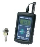
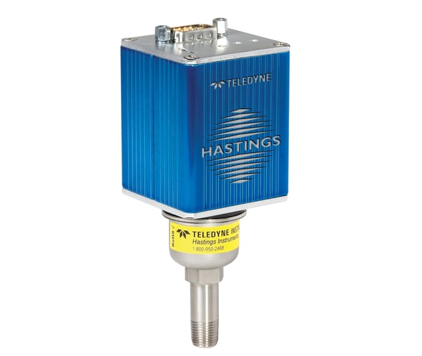
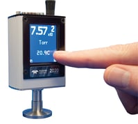The new HVG-2020B from Teledyne Hastings is a great vacuum gauge for this application. The gauge uses two vacuum sensors: a piezoresistive sensor to measure pressures from atmosphere to 10 Torr and a thermal Pirani sensor to measure from 1 Torr to 0.1 mTorr. In between 1 and 10 Torr, the gauge uses a weighted average to ensure a smooth transition between the two sensors. The piezoresistive sensor is gas species independent, so no matter what gas is being backfilled, the piezoresistive sensor gives an accurate measurement. The Pirani sensor’s response is affected by the gas species, but the user can select a gas and the correction is made.

So, the next time you see a neon light, you can think about the vacuum gauge that was probably used to manufacture the gas tube. And if you’re ever in Vegas, check out the Neon Museum!

For more information about any of our vacuum gauges or our complete line of mass flow meters and controllers, we are here to help. You can contact us at hastings_instruments@teledyne.com , Live Chat on our website www.teledyne-hi.com , or call 757-723-6531 (800-950-2468). And to learn more about the HVG-2020B Vacuum Gauge, click the link below, “5 Reasons you need the HVG-2020B Vacuum Gauge.”

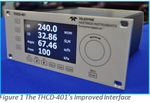Teledyne Hastings is proud to announce our newest 4-channel power supply, controller and display, the THCD-401. The THCD-401 provides both ±15 VDC or 24 VDC to power our mass flow controllers, flow meters, vacuum gauges and pressure transducers. Feedback from connected devices is displayed on the bright, front panel LED display in 6-digit resolution, making open and closed channels easily identified at a glance. The THCD-401 can set a relay point for control of other processes and has a high accuracy of ± (0.02% of Reading + 0.01% of Full Scale). Custom configuring our products to customer needs is our specialty. Your THCD-401 can be factory configured to match the gas, range, units and the output of your instruments for out-of-box functionality.

What’s Improved?

In short, the THCD-401 was designed for exceptional user access and control.  The addition of a circular touch pad simplifies navigation through the unit’s various menu options, while left and right arrow keys allow easy selection of digits to be changed. Calibration is no longer needed for various levels of input voltage and built-in fuses provide additional surge protection.  Back panel communication ports have been streamlined and a USB-C and Ethernet port for serial communication have been added. 

The addition of Ethernet communication provides access to the newest feature that the THCD-401 has to offer; the internal web server! The web server can be accessed by entering the IP address of the THCD-401 into a browser’s address bar (requires static IP address configuration on the network prior to use). While the web server feature works best in Mozilla™ Firefox^®, it can be accessed via any browser you choose.  Figure 2 shows the web server interface with applications along the top navigation bar and a live data stream for remote read.

The web server allows you to name channels and adjust the range or units based on your device and the full scale (V) voltage output that it sends. This enables users to see the flow rate of a flow controller or meter, as well as the ability to OPEN/CLOSE all channels at the click of a button. Other applications include linearization, setting of a relay point and finding the total amount of gas that has passed through the device using the totalizer function.

It should be noted that while all these advanced features are available via the web server (Ethernet) connection, the THCD-401 also offers direct access to each via the front panel display menus using the circular touch pad.  This allows for quick and convenient setup of the channel’s full scale and range(V) for new devices.

If a relay point has been tripped, it will be indicated to the left of the channel’s name on the THCD-401 display. The display will also show the current mode of the set point, if it is not configured in AUTO mode. In OPEN mode, the set point outputs a voltage greater than the full scale of the device. In CLOSED mode the set point outputs a voltage less than the minimum output voltage of most devices. AUTO mode is dependent on the user defined set point configured through the THCD-401 physical buttons, digital communication or external input. 

More Information:

The THCD-401 was designed to be a highly flexible and multi-featured process display controller that can be panel mounted and capable of interfacing to an assortment of meters, controllers and gauges.  A powerful upgrade from the previous THCD-400 model, the THCD-401 adds digital communications, a bright LED display and a variety of customizable options to an already time-tested platform. To learn more about the
THCD-401 or any of our other vacuum and flow products, contact us at hastings_instruments@teledyne.com, call 1-800-950-2468, or click the button below.

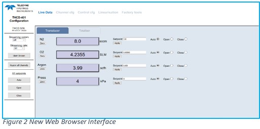
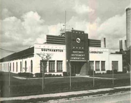The early part of the 1950’s was prosperous for Hastings due in part to the demand for the Raydist and large military contracts as a result of the Korean War. Sales nearly tripled between 1950 and 1953 and there were almost 200 employees.  Hastings had outgrown its space yet again and expanded to a 14,000 square foot building on Newcomb Avenue (current day location for Teledyne Hastings).  The building was originally used as a car barn for street cars, then as a World War I armory and eventually as a manufacturing plant for ladies clothing.

With the new location, other changes were happening as well.  Hastings entered into a joint venture to supply Raydist services for the petroleum industry in the Gulf of Mexico thus creating Offshore Raydist, Incorporated. Another company was formed out of Hastings at this time, Raydist Navigation Corporation (RNC).  RNC was set up to handle the leasing of Raydist equipment outside of the Petroleum industry.

During this period, most of the focus was on Raydist and trying to establish itself in new fields.  One area was to have the Raydist on the S.S. United States.  This superliner promised to be the fastest passenger liner in the world and would serve as a troop transport in the event of war.  Because of personal relationships, Hastings could test and prove that Raydist was the superior system of conducting the tests at a measured-mile course.  The test would use a specially-designed buoy which could be cast overboard and allowed to float freely during the trials.  The relay equipment would be installed in the buoy, while the S.S. United states would carry the master station.  Raydist would then record the liner’s speed as it steamed directly toward or way from the buoy.  The tests proved to be successful and resulted in the Raydist being approved for use on the S.S. United States.  This success lead to many other shipyard opportunities for Hastings.  Within a few years, Raydist dominated the sea trial business in the United States.

Raydist was also gaining momentum in the Hydrography and oil prospecting industry due to positive publicity from the Norfolk Corps of Engineers.  This publicity resulted in the first foreign Raydist sale in early 1951 to be used in charting the waters off Mozambique in southeast Africa.

During this time, Hastings completed a Raydist system for the All-Weather Flying Division of the Air Force.  It was to be used at Wright-Patterson Air Force Base in Dayton Ohio to test the accuracy of radar and other blind landing systems. Later that year, an automatic plotting board was developed to supplement the Raydist system.  The demonstration of this new product was a big event.  The board plotted a plane’s path as it performed skywriting maneuvers spelling HICO across the sky.

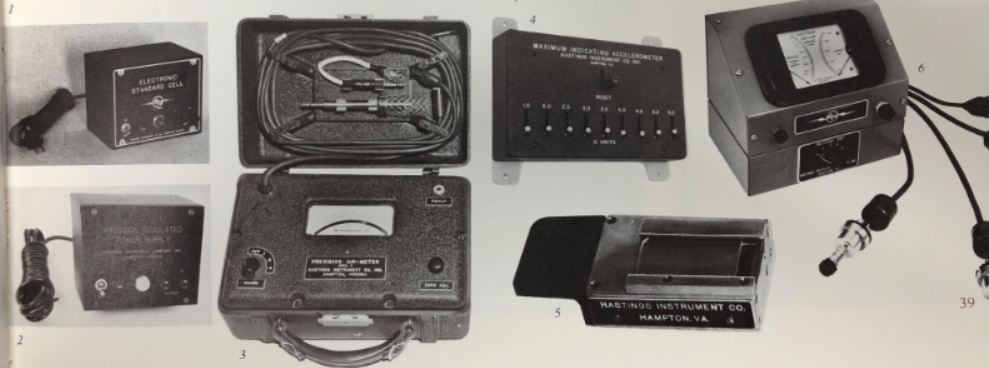
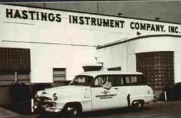A small percentage of Hastings business during the early 1950’s was for instrument sales.  The most important of these products were the air-meters, vacuum gauges, flow meters, accelerometers and an electronic standard cell. In order to grow this part of the business, Hastings decided to set up a manufacturer’s representative program.  By the end of 1953, Hasting’s was looking forward to seeing this manufacturer’s representative program vastly increasing instrument sales.

(Image on right is the first Manufacturer Representative's car outfitted with Hastings products.)

For more information on Teledyne Hastings be sure to visit our website www.teledyne-hi.com or contact us

Information for this blog was derived from “The Story of Hastings-Raydist” book by Carol Hastings Sanders 1979

By 1947, the Hastings Instrument Company could count many successful projects.  Their list of products included the following:

• Raydist Navigation System
• Magnetic Switch and Coil
• Maximum Recording Accelerometer
• Visibility Meter

While the list of projects was impressive, the company wanted to grow their profits further. Charles Hastings decided to look at his business model and make some changes.  The company needed to raise capital for further development in order to become a sizeable company. Growth would give the company the ability to attract and close larger contracts.  To do this, Hastings decided to incorporate the business and offer 3500 shares of stock.  The company charter was received from the Commonwealth of Virginia on Valentine’s Day 1947. 

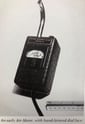After several sales pitches and demonstrations, Hastings received two large contracts for Raydist. Along with these two contracts, the company was busy building Air-Meters for commercial sales.  Before selling the Air-Meters, the instruments needed to be calibrated.  In those early days, calibration was done by driving down the road holding a probe out the window while someone in the passenger seat held the Air-Meter.  When the car reached 5, 10, 15 etc… mph the passenger would make a note on the blank dial face and then return to the house where they would neatly letter the dial face.

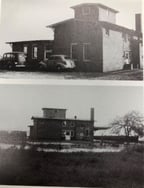During this period of growth, Hastings realized that it was time to find a new location for the business.  By now, there were 17 people working elbow-to-elbow at the Hastings’ home and that could not continue.  The company settled on temporary location in an old brick distributorship building that had a leaky roof and flooded at spring tides, but it was at the price they could afford.

By the spring of 1948, several Raydist contracts were in the works. Air-Meters continued to sell very well, and several instruments were about to be introduced.  That same year, the Hastings Company also moved into a more permanent building for its now 75 employees, which would grow to 118 by 1950.  To secure the company and continue to make profits, Hastings realized he needed to produce a Raydist for commercial use.  The company achieved this goal in 1950 with a sale to the Norfolk Corps of Engineers for hydrographic surveys and channel dredging.

By 1950, the line of Hastings Instruments increased to the following:

• Air-Meter
• Precision Air-Meter (for higher ranges and more accurate readings)
• Maximum Indicating Accelerometer
• Voltage-regulated Power Supply
• Electronic Standard Cell
• Vacuum Gauge

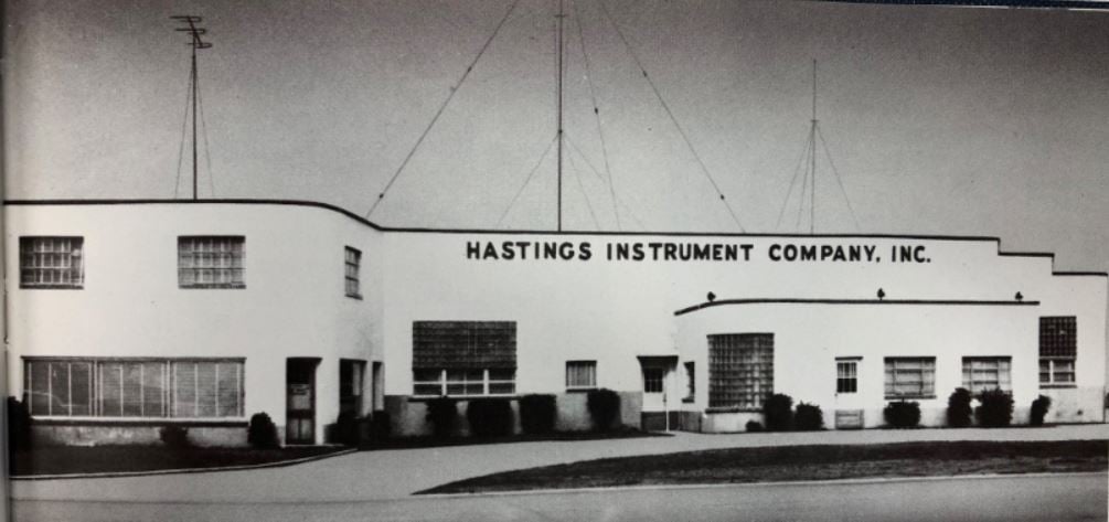
I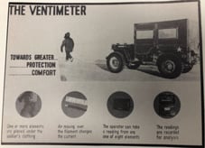n addition to the list of commercial instruments above, Hastings developed specialized instruments for specific customers. For example: the “Ventimeter” was used by the army to measure ventilation in clothing to keep wearers comfortable under extreme weather conditions.  The Hastings Company was now growing fast and generating handsome profits for its stakeholders.

For more information on Teledyne Hastings be sure to visit our website www.teledyne-hi.com or contact us

Information for this blog was derived from “The Story of Hastings-Raydist” book by Carol Hastings Sanders 1979

Recently, I learned that certain smartphones contain an actual pressure transducer. I shared this info with a friend who insisted that the phone was not really measuring pressure, but was instead using the internet to download the pressure based on the phone’s location. Now, I had to prove them wrong.

So, I did what I thought was the obvious proof… I placed my phone in a small test chamber (i.e. a bell jar as shown in the photo below), and then pumped the system down to show that the readings were, in fact, generated locally. I captured this all on video - see below.  Note: It was hard to get a good image of the phone inside because of the protective cage surrounding the glass bell jar.

I used a free barometer app to get the pressure readings. In addition to a dial type readout, the app gives a nice trend line (pressure vs. time). Also, the app allows the user to adjust the time scale. During a recent flight, I used the app to record changes in cabin pressure. (My ears are also painfully good at detecting swings in cabin pressure!)

Now, you may be wondering why a smartphone would include a vacuum/pressure transducer. In addition to using the changing barometric pressure as an indication of weather, the pressure transducer readings can be used to provide the user’s altitude when hiking, cycling, or climbing. The formula to convert pressure to altitude at low altitudes is fairly linear. 

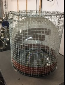
So, it is true that you may be able to use your smartphone to measure vacuum in your system. However, we would like to suggest an easier way… check out our new HVG-2020A (“2020 Vision”) vacuum gauge. This gauge measures from just above atmospheric pressure (1000 Torr) to below 1 Torr with an accuracy of ±(0.1% of Reading + 0.5 Torr).

The gauge features an optional color touchscreen display which has several different modes including pressure vs. time. It provides analog output (0-5 VDC, 0-10 VDC, 4-20 mA,…) as well as digital output (RS232, RS485, USB) and with our FREE Windows™ software, it is super easy to collect and store data.

For more information about any of our vacuum gauges or our complete line of mass flow meters and controllers, we are here to help. You can contact us at hastings_instruments@teledyne.com  or call 757-723-6531 (800-950-2468) or click the button below.

In September 1944, the Hastings Instrument Company started to take shape.  For quite some time, Charles & Mary conducted the business out of their home.  They received their first order in December from the Naval Aircraft Factory in Philadelphia for $800.  The order was for a rotary magnetic switch for commutating electrical circuits. 

The following month, Charles built his first heated thermopile anemometer, which he called the Air-Meter.  This Air-Meter was based on ideas he had had in 1940 for making a thermopile instrument to measure aircraft speed.  It also incorporated his invention of a way to make a thermopile compensated for both temperature and rate of change of temperature. He decided to name his radio ground speed system by combining the first syllables of the words “radio” and “distance” to form “Raydist”.

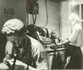Business continued to grow.  Seventeen employees would arrive at the Hastings home around 7pm on Monday, Wednesday and Friday to work on their electronic projects (see image on right).  During the day, Mary would take care of miscellaneous projects.  On one occasion, Mary agreed to have some Raydist cabinets painted by the time Charles came home.  Unfortunately, the air compressor was out of air so Mary came up with another plan.  She would take the car to the nearby service station and put as much air in the tires as she could without them bursting.  She would then drive back home, attach her paint sprayer to the tires, and paint the Raydist cabinets until her tires were almost flat.  She did this several times to complete the project before Charles came home.  The business activities took a toll on the Hastings home. The roof leaked and needed to be replaced from all the antennas mounted to it (see image on left), the driveway needed to be replaced from the damage of delivery trucks, Mary’s oven smelled like paint which caused some challenges when meal time came.

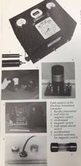
In January 1946, Hastings received their first order for a Raydist.  The Air Material Command at Wright Field in Cleveland Ohio wanted a single-dimensional Raydist system to use during aerial photography and mapping.  The final product was hand-delivered by Charles himself in October. (see image on right and below)

This Raydist order was the largest order Hastings had ever received and he felt that once they were paid for it all, their troubles would be over. 

For more information on Teledyne Hastings be sure to visit our website www.teledyne-hi.com or contact us

Contact Us

Information for this blog was derived from “The Story of Hastings-Raydist” book by Carol Hastings Sanders 1979

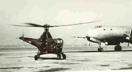
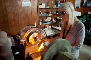
This year, 2019, marks the 75^th anniversary of Hastings Instruments and we will be celebrating all year long by discussing some of our past while focusing on our future. This month, I’d like to tell you a little about our glass shop.

In 1966, Hastings-Raydist purchased the Robert H. Work Company. Work had been a supplier of glass parts for Hastings. The company was then moved into the Hastings plant. At the new location, glass workers began to produce scientific glassware under the Hastings label. Product catalogs in the late 60s and early 70s included McLeod vacuum gauges, calibrated gas leaks, and Pyrex vacuum gauge tubes.

Today, we still use our glass shop to build the Hastings Reference Tube. A reference tube is an evacuated, sealed vacuum gauge tube accurately marked at a specific pressure. It is electrically equivalent to our most popular vacuum gauge tube families.

A reference tube can be used with several of our thermal vacuum gauge instruments including the HPM-4/5/6, the VT and CVT, the DVT and DCVT, and even the DAVC controller. 

How is it used? Simple, you just plug in your reference tube and compare the reading from your instrument with the number that is shown on the reference tube label. 

So the reference tube tells you that your electronics and cabling are working correctly. Note that a reference tube will not directly tell you anything about the state of your gauge tube. But through process of elimination, you can often determine that the gauge tube needs to be replaced. You can learn more about troubleshooting thermocouple vacuum gauges here:

 https://info.teledyne-hi.com/thermocouple-vacuum-gauges-best-practices-webinar-recording?

As noted in the table above, the reference tubes, like the gauge tubes, are color-coded. And reference tubes can be sent back to us to be recertified which many folks do on an annual basis.

Next, let’s discuss a little about what is going on inside of a reference tube. Sometimes people will ask if we adjust the pressure inside the tube to allow it to read a certain value – we do not. In other words, if you could measure the pressure in the sealed-off tube, it would not be the pressure reading that is stated on the side of the reference tube. While a reference tube does have the same thermopile sensor arrangement, it is simply trimmed to give a particular reading when powered by the correct heater voltage.

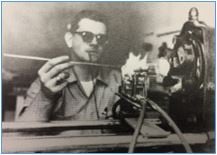
We are proud of our long history of quality craftwork, not only in the glass shop, but throughout all of our vacuum and thermal mass flow product lines here at Teledyne Hastings. The same tradition of quality goes into our newest products including the 300 Vue line of mass flow controllers and the HVG-2020 Vision line of vacuum gauges. You can learn more about our products by visiting www.teledyne-hastings.com

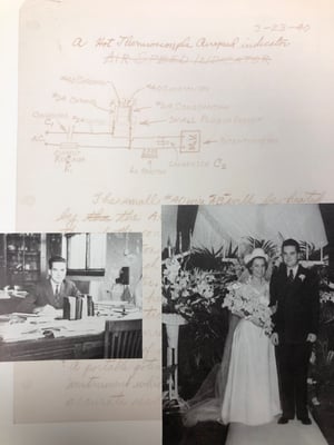Ever wonder where the idea or dream of Hastings originated?  Well as part 1 of our anniversary year blog posts, we thought this would be a good place to start.  Charles Hastings at the age of 10 was bitten by the radio bug and began to build and experiment with radio gear.  In 1930, at the age of 16, Charles Hastings found an opportunity to fund his experiments by fixing other people’s radios.  Many families had radios at this point, but they were very unreliable and frequently needed minor repairs.  Charles would fix radios to earn money to buy parts for his own experiments.

Soon, Charles moved on to building transmitters and enlisted the help of his high school friend, Raymond Doyle.  Their first success was when Charles spoke into a microphone and Ray heard the broadcast from his aunt’s house which was down the street. Unfortunately, the broadcast covered the entire spectrum of commercial radio broadcasting, so the entire neighborhood received the broadcast as well instead of their favorite radio programs.

After this first broadcast mishap, Hastings decided to go back to radio repair.

Charles Hastings went on to attend John Hopkins University and majored in Electrical Engineering.  Upon graduation, he was offered a position as Junior Scientific Aide with the National Advisory Committee for Aeronautics (NACA) in Hampton, Virginia. In 1939, Mary Comstock joined NACA as a mathematician and Charles was quick to ask her out for a date.  They were married within a year.

Working at NACA proved to be quite rewarding to Charles.  He came up with an idea for a magnetically operated reed switch for the spin tunnel section in order to flip the controls in its free-spinning airplane models.  This moved on to finding accurate methods to measure the speed of aircraft.  In 1940, Charles did just that, he came up with an idea for an airspeed indicator using a heated thermopile.  The idea was tested later that year at Langley Field in measuring the speed of planes.  This was the first continuous-wave heterodyne system ever used for speed measurement and was names the NACA Radio Ground Speed System.

His work continued at the NACA for a few years, but Hastings became restless and wanted to be on his own.  He felt that the work he had done with Radio Ground Speed System had more potential in the measurement of distances.  Initially Charles Hastings only wanted to create ideas for commercial products and sell the rights to others in exchange for royalties.  Hastings longtime friend James Benson was interested in being a part of this new.

Hastings Instruments Company was born in September 1944.

For more information on Teledyne Hastings be sure to visit our website www.teledyne-hi.com or contact us

Information for this blog was derived from “The Story of Hastings-Raydist” book by Carol Hastings Sanders 1979

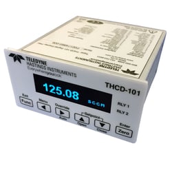Teledyne Hastings is proud to announce the release of the THCD-101 single channel power supply, controller and display.  The THCD-101 can be used to operate a wide variety of mass flow meters and controllers as well as vacuum gauges and pressure transducers. The THCD-101 uses bright OLED digits which makes the display easy to view, even from a distance. The THCD-101 is extremely versatile in its configurable range and can be set up to display any unit of measurement through customizable alphanumeric characters.  The power supply provides stable ±15 VDC and +24 VDC levels which can be used to operate a variety of measurement and control instruments. The display and readout features a high accuracy of ±(0.02% of Reading + 0.01% of Full Scale).  The user can also set relay alarms for the control of other processes.  The THCD-101 is configured at the factory to match the user’s requirements for range & units so it is ready to use right out-of-the-box.

The main screen of the THCD-101 display (pictured above) shows the current reading from the connected instrument and measurement units.  If relay alarms have been tripped, they will be indicated on the far right of the display screen.  Lastly, the main screen will show the current mode of the setpoint, if not in AUTO mode. There is an OPEN mode and CLOSED mode.  In OPEN mode the setpoint outputs a voltage greater than the full scale of the device. In CLOSED mode the setpoint outputs a voltage less than the minimum output voltage of most devices.  AUTO mode is dependent on the set point the user commands via either the THCD-101 physical buttons, digital communication, or external input.

The menus pack several features into the THCD-101 while still ensuring ease of operation for the user.  Through the intuitive menus, the user can enter a setpoint, change the full-scale range & full-scale output voltage (5 VDC or 10 VDC), program alarm relays for process control, restore factory defaults, and many other helpful options. 

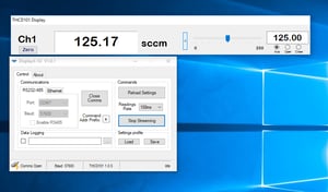The THCD-101 now includes digital communication via a USB ‘C’ connection or Ethernet (TCP/IP).  When the power supply is connected via Ethernet, the THCD-101 provides a web server for operation and instrument configuration. The web server can be accessed by entering the IP address of the device into a browser address bar (requires static IP address configuration on the network prior to use). This allows the user control of various settings within the device and to read the devices current reading. Note that the IP Address can be changed through the menus of THCD-101.  In addition to the THCD-101 web server, standalone DisplayX software can be downloaded free of charge from the Teledyne Hastings website.  Should the user need to change the THCD-101’s setup, the DisplayX software or Ethernet web server is extremely helpful in streamlining this process.

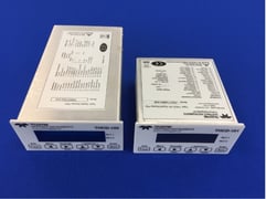As outlined above, the THCD-101 contains all the great features of the legacy THCD-100 while adding new and improved features such as USB & Ethernet digital communications and a bright OLED display.  Even with these powerful additions, the instrument keeps the same 1/8 DIN size while offering a shorter depth than the previous display & readout!

The THCD-101 is a very flexible and multi-featured process display controller that is capable of interfacing to an assortment of meters, controllers, and gauges. To learn more about the THCD-101 or any of our other vacuum and flow products, contact us at hastings_instruments@teledyne.com, call 757-723-6531 (800-950-2468), or click the button below.