Note: The content of this blog was updated February 4, 2023 to provide more information for the reader.
The applications engineers here at Teledyne Hastings discussed topics for our blog. We all agreed that one of the more frequent questions fielded, involves the units used to measure vacuum levels. We find that the technicians who use their vacuum system daily often seem to develop a sixth sense about the “health” of their systems. They know something isn’t quite right when the base vacuum pressure (or rate of pressure change) is not what they expect. So, when vacuum pressure measurements are inconsistent from batch-to-batch, that is the time when the user stops to ask the meaning behind the data that their vacuum measurement instrumentation is providing.
Measuring Vacuum Pressures
A vacuum exists when there is negative pressure, or when there is system pressure that is less than atmospheric pressure. Manufacturing processes generate different levels of vacuum when operating at peak efficiency for a given vacuum application that are measured using a vacuum gauge. Absolute vacuum is the absence of all matter. Atmospheric pressure, also known as barometric pressure, is the pressure due to earth’s atmosphere. Atmospheric pressure is 760 Torr or 14.696 psia at sea level and changes with altitude. The vacuum pressure scale is book-ended by absolute vacuum pressure in the “ultra-high” vacuum range and atmospheric pressure at the “rough” vacuum range. It should be noted that absolute vacuum, or perfect vacuum, is never truly attained.
Most users know that vacuum is commonly measured using units of pressure. There are a few different systems of pressure measurement, and this blog will discuss those most used. In Armand Berman’s book, Total Pressure Measurements in Vacuum Technology, pressure unit systems are divided into two categories: “Coherent Systems” and “Other Systems”.
Common Units of Vacuum
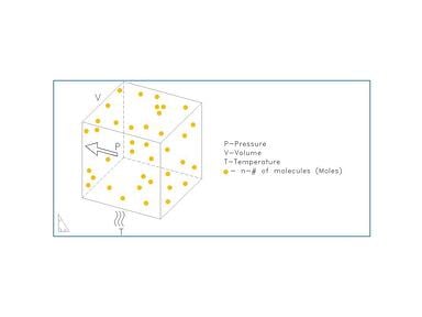
“Coherent Systems” of units are based on the definition of pressure (P) as the force (F) exerted on a chamber wall per unit area (A). P = F/A. The International System of Units, or SI units, is commonly used for pressure measurement. http://physics.nist.gov/cuu/Units/units.html The SI unit for pressure is the Pascal (Pa), and it is interesting to note that NIST (National Institute of Standards and Technology) published papers are always required to use SI units. Again, the SI unit for pressure (force per unit area) is the Pascal. 1 Pa = 1 N /m2.
As a unit of pressure, the Pascal is not always convenient to use because vacuum systems often operate in pressure ranges where collected data results in large numbers. For example, near atmospheric pressure, we would measure approximately 100,000 Pa. So, a more convenient unit, the bar, was developed. (1 bar = 100,000 Pa)
Moving lower in pressure, it is very helpful to then use the mbar (1 mbar = 0.001 bar), which has become the predominate unit of measure in Europe, as the basis for describing pressure levels. As a specific example, look at the base pressure specification of a turbo pump, which will typically be given in terms of mbar (e.g., Base Pressure < 1 x 10⁻¹⁰ mbar).
“Other Systems” of units include the Torricelli system, which is based on an experiment (shown in the diagram below) conducted by the Italian scientist, Evangelista Torricelli. In this experiment, the pressure exerted on the mercury can be shown to be P = hdg, where h is the height of the mercury column, d is the density, and g is the acceleration due to gravity.

By measuring the mercury column height, the pressure can be determined. The Torr unit (named after Torricelli) has been defined as 1 millimeter of mercury (1 Torr = 1 mmHg). This unit, as well as the use of the mTorr unit (1 mTorr = 0.001 Torr), is commonly used in the United States. Historically, pressure was sometimes described in terms of “microns”, which simply meant a mercury column height of one micron (1x10⁻⁶ m). Note that the micron and the mTorr are the same.
Lastly, it should be noted that occasional confusion arises between the use of different, but seemingly similar, units of pressure. As explained above, the mbar and the mTorr are not the same. One mbar has the same order of magnitude as one Torr (1 mbar = 0.75 Torr).
Unit Conversions
The table below gives some conversion values between various commonly used units of pressure and vacuum. A useful website for conversions:
http://www.onlineconversion.com/pressure.htm
| |
Pa
|
mbar
|
Torr
|
mTorr (micron)
|
Atm
|
|
1 Pa =
|
1
|
0.01
|
0.0075
|
7.50
|
~ 10-5
|
|
1 mbar =
|
100
|
1
|
-.75
|
750.06
|
~ 10-3
|
|
1 Torr =
|
133.3
|
1.333
|
1
|
1000.0
|
~ 10-3
|
|
1 mTorr (micron) =
|
0.1333
|
0.00133
|
0.001
|
1
|
~ 10-6
|
|
1 Atm =
|
101,325
|
1013.25
|
760
|
760,000
|
1
|
Absolute Pressure and Gauge Pressure
In conclusion, keep in mind that vacuum measurements can be referenced to ambient pressure, gauge pressure measurement or absolute pressure measurement (perfect vacuum). An absolute pressure measurement is referenced with respect to absolute vacuum. Absolute pressure will often be designated by the letter “a” after the unit of measure; “psia.” As an example, an absolute pressure reading of 30 psia (pounds per square inch absolute) is a pressure that is 30 psi above vacuum. It is important to understand that there is no negative absolute pressure. There are some
Gauge pressure measurements are measured relative to the ambient atmospheric pressure. Relative, or gauge pressure, will often be designated by the letter “g” after the unit of measure; “psig.” As an example, 30 psig is a gauge pressure that is 30 psi above ambient atmosphere (typically 14.7 psia at sea level). In this example the gauge pressure, 30 psig, is equal to an absolute pressure of 44.7 psia.
What is a vacuum system?
A vacuum system can consist of multiple a vacuum pumps and vacuum gauges attached to a tank that is designed to measure below atmospheric pressure. The vacuum pumps reduce the air pressure inside of the tank to the pressure range that the vacuum pump is rated for. Different vacuum pumps bring the vacuum pressure to different levels depending on the strength of the vacuum pump.
Attached to the tank is usually at least one vacuum pressure gauge. An application may require another type of vacuum gauge to measure a different pressure point. An example of this would be using a piezo pressure gauge and a Pirani pressure gauge to have a larger range of the vacuum pressure measured. A piezo vacuum gauge would be used to measure the rough vacuum range around atmosphere and the Pirani could be used to measure below 1 Torr in the mTorr range. There are vacuum gauges that use technologies from different vacuum gauges to create a combination vacuum gauge to measure vacuum pressure across a wider pressure range. Teledyne Hastings combines both the Pirani and piezo technologies to make the HVG-2020B vacuum pressure gauge.
Vacuum Gauges Poster
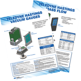 |
Vacuum Gauges
Free Poster
Unit Conversions and More

|
Original Content posted Sept 22, 2014
FAQ Corner - Units for Vacuum Measurement
an overview of units used to measure pressure
Earlier this year, the applications engineers here at Teledyne Hastings discussed topics for our blog. We all agreed that one of the more frequent questions that we discuss with folks involve the units used to measure vacuum levels. We find the technicians who use their vacuum systems daily often seem to develop a sixth sense about the “health” of their systems. They know something isn’t quite right when the base pressure (or rate of pressure change) is not what they expect. So, when pressure measurements are not consistent from batch to batch, that is the time when the user stops to ask the meaning behind the data that their vacuum measurement instrumentation is providing.
Now, most users know that vacuum is commonly measured using units of pressure. There are a few different sets of pressure units, and this blog will discuss the more commonly used ones. In Armand Berman’s book, Total Pressure Measurements in Vacuum Technology, pressure unit systems are divided into two categories: “Coherent Systems” and “Other Systems”.
Coherent Systems of Units are based on the definition of pressure (P) as the force (F) exerted on a chamber wall per unit area (A). P = F/A. The International System of Units, or SI units, is commonly used for pressure measurement. http://physics.nist.gov/cuu/Units/units.html The SI unit for pressure is the Pascal (Pa). It interesting to note that at NIST (National Institute of Standards and Technology), published papers are always required to use the SI set of units. Again, the SI unit for pressure (force per unit area) is the Pascal. 1 Pa = 1 N /m2.
Now, the Pascal as a unit of pressure is not always the most convenient because vacuum systems are often operating in a range of pressures where we would need to collect data using large numbers. For example, near atmospheric pressure, we would measure approximately 100,000 Pa. So, a more convenient unit, the bar, has been derived. (1 bar = 100,000 Pa)
Moving lower in pressure, it is very helpful to then use the mbar (1 mbar = 0.001 bar). So many vacuum users, especially in Europe, use the mbar as the basis for describing pressure levels. As a specific example, look at the base pressure specification of a turbo pump, it will be given in terms of mbar (e.g. Base Pressure < 1 x 10⁻¹⁰ mbar).
Another system of pressure units is based on the Torricelli experiment (shown in the diagram). In this experiment, the pressure exerted on the mercury can be shown to be P = hdg, where h is the height of the mercury column, d is the density, and g is the acceleration due to gravity.
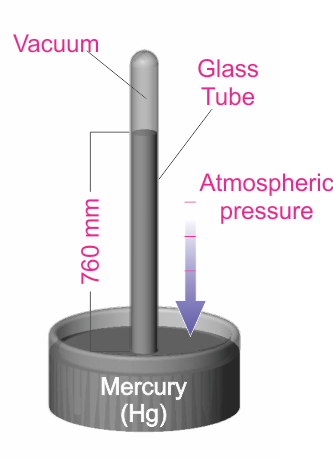
By measuring the mercury column height, the user can determine the pressure. The Torr unit (named for the Italian scientist Torricelli) has been defined to be 1 millimeter of mercury (1 Torr = 1 mmHg). This unit is very common, especially in the United States. It is also common to use the mTorr (1 mTorr = 0.001 Torr). Many years ago, pressure was sometimes described in terms of “microns”, which simply meant a mercury column height of one micron (1x10⁻⁶ m). Note that the micron and the mTorr are the same.
One last word about the units used to measure vacuum: on occasion, there is confusion between pressure units. As we have seen above, the mbar and the mTorr are not the same. One mbar has the same order of magnitude as one Torr (1 mbar ≈ 0.75 Torr). The table below gives some approximate conversion values. A useful website for conversions:
http://www.onlineconversion.com/pressure.htm
|
|
Pa
|
mbar
|
Torr
|
mTorr (micron)
|
Atm
|
|
1 Pa =
|
1
|
0.01
|
0.0075
|
7.50
|
~ 10-5
|
|
1 mbar =
|
100
|
1
|
0.75
|
750.06
|
~ 10-3
|
|
1 Torr =
|
133.3
|
1.333
|
1
|
1000.0
|
~ 10-3
|
|
1 mTorr (micron) =
|
0.1333
|
0.00133
|
0.001
|
1
|
~ 10-6
|
|
1 Atm =
|
101,325
|
1013.25
|
760
|
760,000
|
1
|
Douglas Baker is the Director of Sales & Business Development of Teledyne Hastings. Antonio Araiza prepared the Torricelli experiment drawing. Antonio is the head of Technical Documentation at Teledyne Hastings (and is among the best soccer referees in the Commonwealth of Virginia).

 As we say good-bye to John Glenn, it is a good time for Teledyne Hastings to recall with pride our company’s and our city’s connection to this great American hero. Now, many people know that John Glenn was the first American to orbit the earth. But most people don’t know that the original seven Mercury astronauts, including John Glenn, received their original spaceflight training in 1959 at NASA-Langley in Hampton Virginia which is also our home for Teledyne Hastings.
 The Hampton Roads area of Virginia has memorialized several landmarks to commemorate Project Mercury. There are several bridges in the city of Hampton which are named for the astronauts. “Military Highway” was renamed to Mercury Boulevard. And, in Newport News, the Denbigh branch of the Newport News Public Library System is the “Grissom Library”.
  And speaking of mathematicians at Langley, there is a movie “Hidden Figures” (released December 25, 2016), which tells the story of three female mathematicians who were part of the computer pool. Which brings us back to John Glenn. In the early days of computers, engineers did not always trust the results of the electronic data processors. The computer pool, in other words, human mathematicians, were used to crunch through complex calculations. Before his historic flight in 1962, Glenn requested that one of these computer pool women, Katherine Johnson, verify the results of the computer. The contributions of these women to the space program was remarkable.
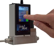 Teledyne Hastings is proud to release our newest, most advanced, line of digital flow meters and flow controllers - the 300 Vue. In this blog, we will discuss the three types of Input/Output (I/O) that can be used with the 300 Vue. These are: Analog, Digital, and Touchscreen Display.
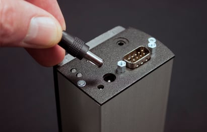
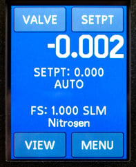
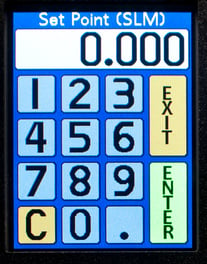


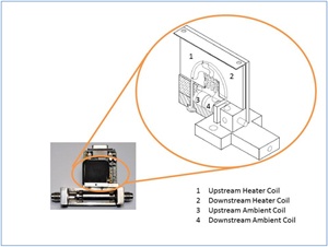 In our previous blog, we showed a cutaway of a thermal mass flow meter. Now let’s take an inside look at the 300 series flow sensor:
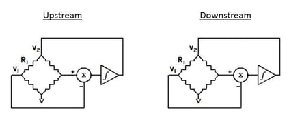 Two identical Wheatstone resistance bridges are formed from the two pair of coils (see image on right).
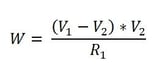
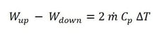
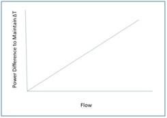 Now, here is the best part: the mass flow rate is directly proportional to the power difference. In other words,
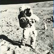 The history of the Hastings Instruments Company stretches all the way back to 1944. Next year, Hastings will celebrate its 70th birthday. But while we are in a corporate history mood, it might be fun to recall everybody’s favorite Hastings’ story: In 1967, Hastings vacuum sensors were designed to travel to the moon and back. One of the objectives of the Apollo missions was to bring lunar samples back to earth. Special boxes, fitted with Hastings vacuum thermocouples were designed and built by Oak Ridge National Labs. Each box was required to be vacuum sealed; the Hastings thermocouple ensured that the seal was good before launch, and after splash down. The box and sensor worked perfectly. Today, the thermopiles from the Apollo 14 mission are on display on a wall between one of the company’s conference rooms and a hallway. A magnifying lens and lamp installed in the display allows visitors to see the vacuum sensor.